Monthly Date Tracker – Tutorial, Part 1

By Rakesh Pal

Do you need to keep track of monthly dates for employees?

Perhaps to mark when a performance review was carried out?

And to easily determine which employees were overdue?

Our Goals:

1. Create a spreadsheet that allows a novice Excel user to track monthly dates for employees, throughout the Fiscal Year.
2. Minimize user error through the use of drop down lists.
3. Be able to customize the start of the Fiscal Year.
4. Be able to create additional options alongside the existing monthly dates
5. Be able to generate a report, to summarize and analyze the data.

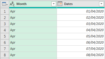
The user data is entered into a Table:

The steps involved:

1. Create a Extra Options Table
2. Create a Date Table
3. Create a User Table
4. Generate a Report

---

1. Create a Extra Options Table

Here’s an overview of the Queries involved with making the Extra Options Table – or ExtraOptionsFromTableBuild as i have named it here. I’ll explain what each of the queries does.

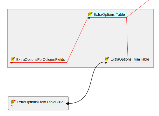
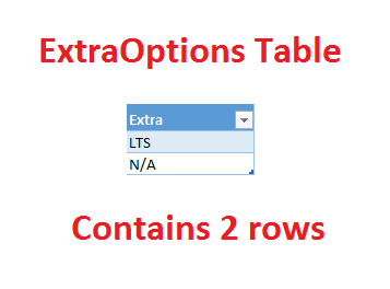
ExtraOptions Table

The ExtraOptions Table is located on the Tutorial sheet.

The User will type in additional options required here.

The Table will be loaded into Power Query and will be amended to the Monthly Drop Down Lists, during the creation of the Date Table.

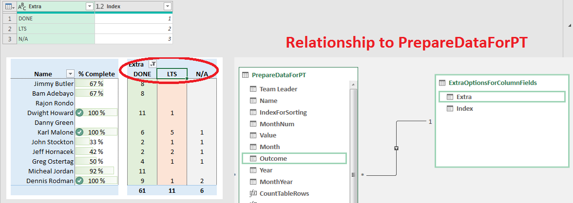
ExtraOptionsForColumnFields

This is a Dimension Table. Its used to create a Relationship to the PrepareDataForPT Fact Table. It’s also used to create Column Headers for our Report.

• Loads in ExtraOptions Excel Table
• Removes blanks
• Inserts a “DONE” row at the beginning
• Creates an Index for sorting

ExtraOptionsFromTable

• Loads in ExtraOptions Excel Table
• Removes any blank rows

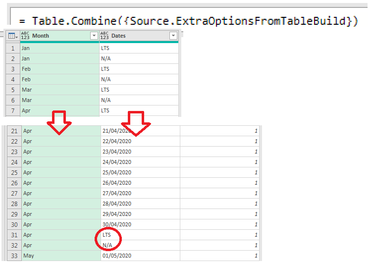
ExtraOptionsFromTableBuild

ExtraOptionsFromTableBuild is later referenced by PrepareDataForPT to create our final Date Table.

• Creates a Table of Months
• For every row, loads in ExtraOptionsFromTable[Extra] Column (List of all Extra Options)
• Expands the lists, to create a Table of Months and Extra Options

---

2. Create a Date Table

Our task is to create a Date Table, which we will later reference in order to create Monthly Drop Down Lists.

Here’s an overview of the Queries involved in making the Date Table, and additional queries that will be used. I’ll explain what each does.

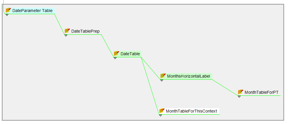
DateParameter Table

The DateParameter Table is located on the Tutorial sheet.

The User will type in the 1st date of the Fiscal Year required and Power Query will reference this in the creation of the Date Table

DateTablePrep

• Loads in DateParameter Table
• Creates a List of Dates (365) from this date onwards.
• Creates a Month name Column

DateTable

After the Date Table is created it’s loaded onto the Data sheet. The Data sheet is hidden by default, to avoid the User breaking the spreadsheet if they accidently edit or remove it.

• Combine our Users Extra Options alongside the existing Dates (Combine the ExtraOptionsFromTableBuild query to this query).
• Group everything by Month name
• Create an Index
• Create a Quarter number – using formula and Index value
• Expand all rows
• Now our dates have a Quarter Number.

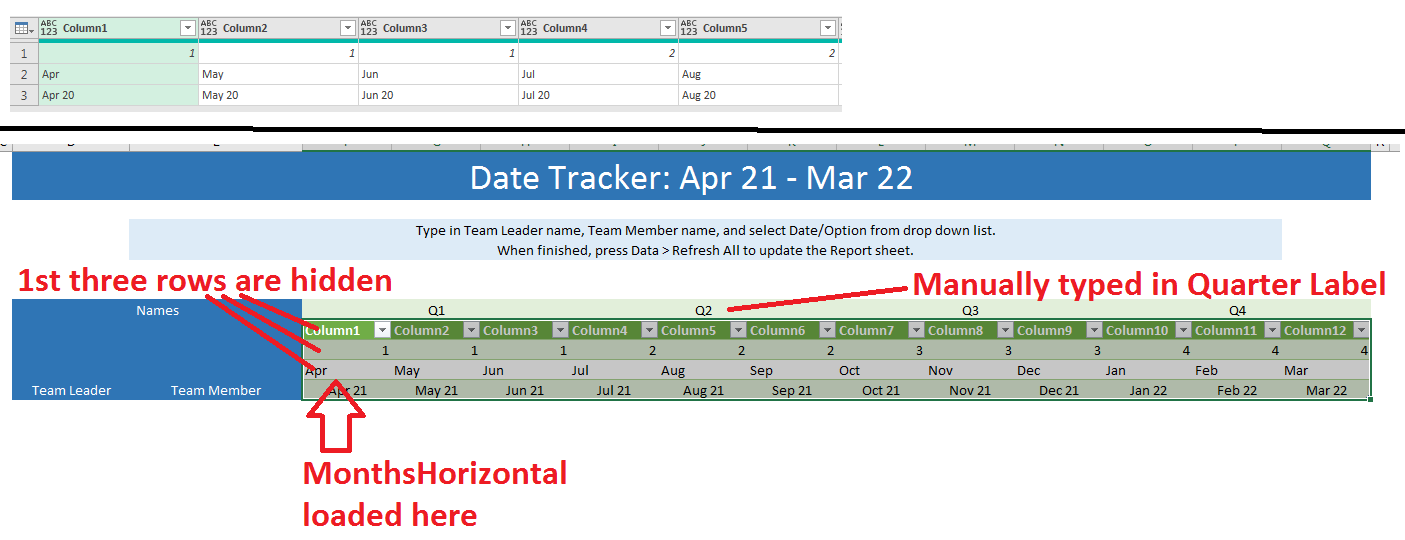
MonthsHorizontalLabel

This is loaded onto the Date Tracker sheet to create Column headers for each Month of the User Table.

• Groups By Month, grabs first row of Date/Quarter, discards others.
• Creates a MonthYear Column, i.e. Jan 20, Feb 20 etc.
• Removes Date Column.
• Transposes rows, so rows become Columns and Columns become Rows.

MonthTableForThisContext

This is a Helper Table. It is used by the PrepareDataForPT Query in order to merge in the Month and Year columns.

• Groups By Month, grabs first row of Date/Quarter, discards others.
• Creates a Year Column
• Removes Date Column
• Create MonthNum Column

MonthTableForPT

This creates Column Headers for our Report PivotTable, on the Report sheet. The Quarter and Month-Year Columns are used.

• References MonthsHorizontalLabel
• Transposes Table, so Columns become Rows, Rows become Columns
• Renames Columns
• Adds an Index for sorting

---

3. Create a User Table

You may recall earlier that we loaded the MonthsHorizontalLabel query onto the Date Tracker sheet as a Table.

We would like the user to be able to enter a Team Member name in an empty cell and then have Drop Down Lists appear for each Month of the Fiscal Year.

To accomplish this we use Data Validation.

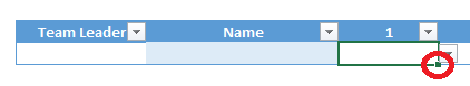
Firstly, let’s unhide the hidden rows of the Table.

Row number 10 contains a 3 letter shorthand for each Month. This is a Helper Row which will allow the Data Validation code to calculate which set of dates we require for this Months Drop Down List. The set of dates is stored on the Date Table, which was loaded onto the hidden Data sheet.

The hidden Data sheet also contain a Table called DaysInMonth, which as you can probably guess, contains the number of days per Month. This is a Helper Table which is referenced by the Data Validation code.

We’re going to create a User Table, which will contain a hidden Default Row.

It’s a standard Excel Table with Columns for Team Leader / Team Member, and numbered Columns from 1 to 12 representing each Month of the Fiscal Year.

We require a Default Row to populate each of the Monthly Columns with Data Validation code, whenever a new row is added to the Table. This will create Monthly Drop Down Lists for the User to select from.

Lets enter the code for Data Validation.

The Data Validation window appears. Select “List” from the Allow drop down box.

Copy and paste the following code into the Source box and press OK. It looks complicated but don’t worry about that for now. (Annoyingly the text box is small and doesn’t allow you to format the code in such a way that it’s easy to read).

=OFFSET(INDIRECT(“DateTable”),MATCH(F$10,INDIRECT(“DateTable[Month]”),0)-1,1,INDEX(INDIRECT(“DaysInMonth”),MATCH(F$10,INDIRECT(“DaysInMonth[Month]”),0),2)+COUNTA(INDIRECT(“ExtraOptions”)),1)

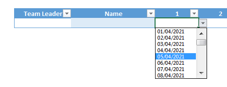
You will now have a Drop Down List appear when you click on the 1st cell of Month 1.

Hover your mouse over the corner of the cell. You’ll see a small crosshair appear (i couldn’t capture it with a screenshot unfortunately).

Whilst holding the mouse button down, drag the cross hair over to the right of the Table, until you reach the right corner of the number 12 cell – then release the mouse button.

This is the Flash Fill feature in Excel, which allows you to quickly copy formulas to other cells.

Now each of the Months has a respective Drop Down List for the User to select a Date or Option.

The Data Validation code uses the OFFSET function to determine which part of the Date Table to use when constructing the Drop Down Lists. In other words, it creates a dynamic range.

I’ll give a breakdown of how the formula works.

Data Validation – Formula

Firstly, an overview of the OFFSET function – and its arguments. This text comes from the Exceljet.net website.

The Excel OFFSET function returns a reference to a range constructed with five inputs:

(1) a starting point,
(2) a row offset,
(3) a column offset,
(4) a height in rows,
(5) a width in columns.

The OFFSET function allows you to create a dynamic range to the Date Table, perfect to construct Drop Down Lists for each of our Months.

Lets examine each argument in turn.

(1) a starting point

Our starting point is simply a reference to our Date Table. In order to use this with Data Validation we have to use the INDIRECT function.

INDIRECT("DateTable")

(2) a row offset

The row offset is which row we would like our dynamic range to begin from on our Date Table.

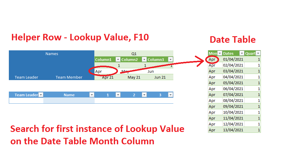
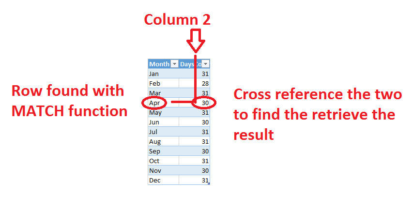
The User Table we created has a Helper Row above each Column which contains a three character shorthand of the respective Month. This is our Lookup Value. Using this we can determine which Row we would like to begin our dynamic range from on the Date Table.

MATCH(
        F$10, 
        INDIRECT("DateTable[Month]"), 
        0)-1,

The MATCH function will return the correct row our Month begins on the Date Table.

F$10 references the Helper row that contains our 3 character Month name – this is our Lookup Value.

INDIRECT(“DateTable[Month”]) is the Column of the Date Table we want to search

0 – Means we require an exact match.

We deduct 1 from the returned row number.

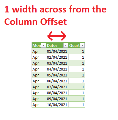
(3) a column offset

1

That’s all – just the number 1.

This is the Column we would like our dynamic range to start from.

Column 1 is the list of dates. We use Base 0 – so Column 1 is 0, Column 2 is 1, and so on.

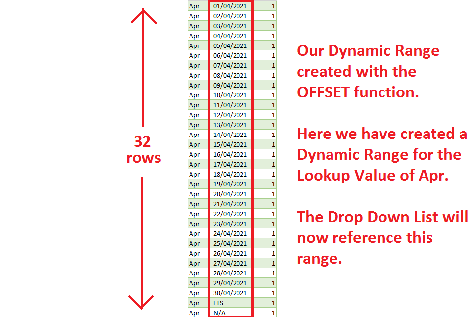
(4) a height in rows

Next we determine how many rows long our dynamic range is from our row offset.

There are two parts

• Retrieve how many days are in the month, using the Lookup Value.
• Count how many options there are in the Extra Options Table.

We add the result of these to determine the amount of rows our dynamic range will contain.

INDEX( 
		INDIRECT("DaysInMonth"),	
		MATCH(
			F$10,	
			INDIRECT("DaysInMonth[Month]"),		
			0		
			),      
		2	
			
		) + COUNTA(INDIRECT("ExtraOptions")),  

The INDEX function allows us to retrieve a value from a range.

In this case our range is the DaysInMonthTable

Firsty, we search the Rows of the DaysInMonthTable with the MATCH function.

• F$10 is our Lookup Value – the 3 character shorthand for the respective Month.
• DaysInMonth[Month] represents the Column we want to search, the Month Column.
• 0 – means an exact match.
• 2 – means the Column to retrieve the value from.

We have found the correct Row the result resides in on the DaysInMonthTable.

INDEX uses Base 1, so 1 means Column 1, 2 means Column 2, and so on.

We have retrieved our answer.

Next, we need to determine how many Rows of options there are on the Extra Options Table.

The COUNTA function returns a count of how many cells there are in a Column, discarding any empty ones.

We have retrieved two values –

• Days in the Month for April, which is 30
• Count of Extra Options Table, which is 2

Therefore our Row Height has a value of 32.

(5) a width in columns

1

Width of Columns is simply 1.

This refers to how many Columns across the range is.

We only require the Dates Column from the Date Table.

Calculated Dynamic Range

Here is the dynamic range our Formula calculated.

It will be available in the Drop Down List for the repsective Month.

Complete the User Table

We have now constructed a Default Row on the User Table.

This row is going to be hidden.

Any time the User creates a new row on the User Table, i.e. adds an employees name, the Month Columns will automatically populate with the Drop Down Lists found on the hidden Default Row.

If the User had access to the hidden row and deleted it, we would lose all of our Data Validation, and the Monthly Drop Down Lists would disappear. Therefore it has to remain hidden.

The completed User Table is loaded into Power Query and the PrepareDataForPT Query modifies it to be used in a Report.

---

4. Generate a Report

Building the Dashboard will be covered in Part 2 of this tutorial.

I hope you found the tutorial useful.

If you have any questions or comments please leave them below.